The derivation of the Black-Scholes-Merton formula is very clearly organized in section 4.5 of Shreve’s Stochastic Calculus for Finance II Continuous-Time Models. It is the most intuitive and clearest way that the author has seen so far. So, this part especially the organization of the article is borrowed from it though not identical.
Evolution of portfolio value
Let ![]() represent the portfolio value at time
represent the portfolio value at time ![]() .
.
We hold ![]() shares of the stock at time
shares of the stock at time ![]() , and put the rest of money in
, and put the rest of money in ![]() . Note that
. Note that ![]() is adapted to the natural filtration of
is adapted to the natural filtration of ![]() . Then, the change of portfolio value is the change in stock plus the interest from
. Then, the change of portfolio value is the change in stock plus the interest from ![]() satisfies the following SDE:
satisfies the following SDE:
(1) ![]()
We plug Geometric Brownian motion ![]() into this equation,
into this equation,
![]()
The SDE of the discounted stock value
(2) 
This equation says that discounting the stock price reduces the mean return rate from
Similarly, the SDE of the discounted portfolio value ![]() is
is
(3) ![Rendered by QuickLaTeX.com \begin{equation*}\begin{aligned}\mathrm{d} (e^{-rt}X(t))& = -re^{-rt}X(t) \mathrm{d} t + e^{-rt} \mathrm{d} X(t)\\&=-re^{-rt}X(t) \mathrm{d} t + e^{-rt}\cdot [rX(t) \mathrm{d} t + \\ & \quad \quad \Delta(t)(\alpha-r)S(t) \mathrm{d} t + \Delta(t)\sigma S(t) \mathrm{d} W(t)] \\& = \Delta(t)(\alpha-r)e^{-rt}S(t) \mathrm{d} t + \Delta(t)e^{-rt}\sigma S(t) \mathrm{d} W(t)) \\& = \Delta(t) \mathrm{d} (e^{-rt}S(t))\end{aligned}\end{equation*}](https://sisitang0.com/wp-content/ql-cache/quicklatex.com-95a435276555f4c79a23e1405fd30e5b_l3.png)
This equation says that the change in the discounted portfolio value is solely caused by the change in the discounted stock price.
Evolution of option value
Let ![]() denote the value of (European) call option at time
denote the value of (European) call option at time ![]() when the stock price
when the stock price ![]() , i.e.
, i.e. ![]() , where
, where ![]() is the strike (contract price to buy stock at maturity). Though
is the strike (contract price to buy stock at maturity). Though ![]() is a deterministic function,
is a deterministic function, ![]() has randomness.
has randomness.
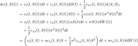
(4) 
The SDE of the discounted call option value is
(5) ![Rendered by QuickLaTeX.com \begin{equation*}\begin{aligned}& \mathrm{d} (e^{-rt}c(t,S(t))) \\ & = -re^{-rt}c(t,S(t)) \mathrm{d} t + e^{-rt} \mathrm{d} c(t,S(t)) \\& = -re^{-rt}c(t,S) \mathrm{d} t + e^{-rt} [ ( c_t(t,S) + \alpha c_x(t,S)S + \\ & \quad \frac{1}{2}\sigma^2 c_{xx}(t,S) S^2 ) \mathrm{d} t + \sigma c_x(t,S) S \mathrm{d} W(t) ] \\& = e^{-rt}[ -rc(t,S) + c_t(t,S) + \alpha c_x(t,S)S + \frac{1}{2}\sigma^2 c_{xx}(t,S) S^2 ] \mathrm{d} t \\ & \quad + e^{-rt}\sigma c_x(t,S) S \mathrm{d} W(t)\end{aligned}\end{equation*}](https://sisitang0.com/wp-content/ql-cache/quicklatex.com-c6d91dcbe1f3a942e9a5b695b40feecd_l3.png)
Equating portfolio and call option values
To hedge the risk of offering the call option, we hold
a portfolio of equal value at all time ![]() . That is equating the portfolio evolution and the call option evolution.
. That is equating the portfolio evolution and the call option evolution.
(6) ![]()
It yields
(7) 
The first equation in (7) is called the delta hedging rule. It says that the number of shares to hold at time
Suppose we could solve the second PDE in (??) with some proper boundary condition. At ![]() we sell the option at price
we sell the option at price ![]() . We create a portfolio using this amount of money (
. We create a portfolio using this amount of money (![]() ) following the delta hedging rule, then the risk of selling the call option is hedged.
) following the delta hedging rule, then the risk of selling the call option is hedged.
We are seeking a continuous solution to the Black-Scholes-Merton partial differential equation
(8) ![]()
with terminal condition
(9) ![]()

![Rendered by QuickLaTeX.com \[\sigma = \sqrt{251 \cdot \mbox{imperical variance}{\log(\frac{S_{n}}{S_{n-1}})}}.\]](https://sisitang0.com/wp-content/ql-cache/quicklatex.com-212843d6c2feb9f6361ca70d55d87648_l3.png)
![Rendered by QuickLaTeX.com \[\sigma = \sqrt{251 \cdot \mbox{imperical variance}{\frac{S_{n}}{S_{n-1}}}}.\]](https://sisitang0.com/wp-content/ql-cache/quicklatex.com-dcbbb8dfdc43f289c8afa9bd230d0425_l3.png)
![Rendered by QuickLaTeX.com \[\begin{aligned}\mathrm{d} S(t) = &\ f_x(t,S(t))\mathrm{d} t + f_y(t,S(t))\mathrm{d} W(t) \\& + \frac{1}{2}f_{xx}(t,S(t))\mathrm{d} \langle t,t \rangle + \frac{1}{2} f_{xy}(t,S(t)) \mathrm{d} \langle t,W(t) \rangle + \frac{1}{2}f_{yy}(t,S(t)) \mathrm{d}\langle W,W\rangle_t\\= &\ ae^{at+bW(t)} \mathrm{d} t + be^{at+bW(t)} \mathrm{d} W(t) \\ & + \frac{1}{2}f{xx}(t,S(t)) \mathrm{d} 0+\frac{1}{2}f_{xy}(t,S(t)) \mathrm{d} 0+\frac{1}{2} b^2 e^{at+bW(t)} \mathrm{d} t \\= & \ (a+\frac{1}{2}b^2)e^{at+bW(t)} \mathrm{d} t + be^{at+bW(t)} \mathrm{d} W(t) \\= &\ (a+\frac{1}{2}b^2)S(t) \mathrm{d} t + bS(t) \mathrm{d} W(t)\end{aligned}\]](https://sisitang0.com/wp-content/ql-cache/quicklatex.com-1fe341fbb442770f267eae1acaa09f4f_l3.png)