Mathematics – Sisi Tang

December 17, 2019March 8, 2021

Feynman-Kac Formula

Feynman-Kac formula connects the solution to a SDE to the solution of a PDE. For example, the Black-Scholes formula is an application of Feynman-Kac.

Let $X(t)$ satisfies the following SDE driven by standard Brownian Motion:

$\textnormal{d}X_u = \beta(u,X_u)\textnormal{d}u + \gamma(u,X_u\textnormal{d}W_u).$

Let $h(y)$ be a Borel measurable function, and $t \in [0,T]$ . Define

$\begin{aligned} g(t,x) := \mathbf{E} [&\int_t^Te^{-\int_t^TV(\tau,X_{\tau})\textnormal{d}\tau}f(r,X_r)\textnormal{d}r \\ &+e^{-\int_t^TV(\tau,X_{\tau})}h(X_T)|X_t = x ] \end{aligned}.$

Then, $g(t,x)$ satisfies PDE

$g_t + \beta g_x + \frac{1}{2}\gamma^2 g_{xx} - Vg + f = 0.$

Proof.

To get an idea of how this formula is proved, we start with a base case. The general case is proved by the same manner with a little more complicated calculation.

Suppose $V=f=0$ .

Let $\mathcal{F}(t)$ be the natural filtration associated with the standard Brownian Motion in the SDE. By the Markov property of the solution to SDE, we have $\forall s \in [0,T]$ ,

$\mathbf{E}[h(X_T)|\mathcal{F}(s)] = \mathbf{E}[h(X_T)|\sigma(X_s)] = g(s,X_s).$

Then, for $0<s<t<T$

$\begin{aligned} \mathbf{E}[g(t,X_t)|\mathcal{F}(s)] & = \mathbf{E}[ \mathbf{E}[h(X_T)| \mathcal{F}(t) ] |\mathcal{F}(s)] \\ &= \mathbf{E}[h(X_T)|\mathcal{F}(s)] = g(s,X_s) \end{aligned}$

Hence, $g(t,X_t)$ is a martingale.

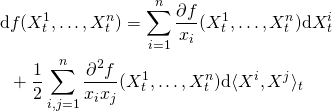
Then, we apply Ito’s formula to $g(t,X_t)$ . Its drift term should be zero because it is a martingale. This leads to the Feynman-Kac PDE.

$\begin{aligned} \textnormal{d}g(t,X_t) & = g_t\textnormal{d}t + g_x \textnormal{d} x + \frac{1}{2}g_{xx} \textnormal{d} X \textnormal{d} X \\ & = [g_t+\beta g_x + \frac{1}{2}\gamma^2 g_{xx}] \textnormal{d} t + \gamma g_x \textnormal{d} W\end{aligned}.$

By setting the $\textnormal{d} t$ term equal to $0$ , we get the PDE:

$g_t+\beta g_x + \frac{1}{2}\gamma^2 g_{xx} = 0.$

For the general case, we only need to factor out the $\int_0^t$ integral and make the integral inside the expectation only contains $\int_0^T$ term. We will get $G(t,X_t)$ is a martingale with $G(t,X_t)$ defined as:

$G(t,x):= e^{-\int_0^tV(\tau,X_{\tau})\textnormal{d}\tau}(g(t,x)+\int_0^t e^{-\int_t^rV (\tau,X_{\tau})\textnormal{d}\tau } f(r,X_r) \textnormal{d}r)$

Similarly, by applying Ito’s formula to above martingale and setting the drift term equal to 0, we will get the result.

March 14, 2019March 15, 2019

Gaussian Mixture Model

Gaussian mixture model (GMM) is a probability model for a mixture of several Gaussian distributions with possibly different mean and variance.

For example, we can model the 100m race time of all grade 12 students in a high school as two normal distributions: one for female students and one for male students. It is reasonable to expect two groups have different mean and may different variance.

When to use Gaussian mixture model?

1. Data has more than one clusters.
In the following picture, the left one models the data with one normal distribution; the right one models the data by two normal distribution, Gaussian mixture model. Obviously, the right one better describes the data.

Pictures are from https://brilliant.org/wiki/gaussian-mixture-model/

2. Each cluster is theoretically normally distributed.

Theory of Gaussian Mixture Model

1. Gaussian distribution in 1 dimension
Since there are several Gaussian distributions in the GMM. We assign an index to each Gaussian distribution: $k$ for $k=1,2,..., K$ where K is the number of clusters. For a given mean $\mu_k$ and variance $\sigma_k$ , the probability density function is

$p_k(x|\mu_k,\sigma_k) = \frac{1}{\sigma_k\sqrt{2\pi}}exp\left(-\frac{(x-\mu_k)^2}{2\sigma_k^2}\right)$

Above $|$ is not the mathematical conditional expectation, but a statistical way of saying we know true parameters $\mu_k,\sigma_k$ in advance.

2. Gaussian mixture model in 1 dimension
The probability density function of GMM is the weighted average of several Gaussian densities:

$p(x|\mu_k,\sigma_k, k=1,2,...,K) = \sum_{k=1}^K w_k \cdot p_k(x|\mu_k,\sigma_k ),$

where $w_k \in [0,1]$ satisfies

$\sum_{k=1}^K w_k = 1$

Plug in the Gaussian density,

$p(x) = \sum_{k=1}^K w_k \frac{1}{\sigma_k\sqrt{2\pi}}exp\left(-\frac{(x-\mu_k)^2}{2\sigma_k^2}\right)$

Note that this is a density function because its integral on $\mathbb{R}$ is 1.

3. Gaussian mixture model in n-dimension
Let $x \in \mathbb{R}^n$ be an n-dimension multivariate Gaussian random variable with mean vector
$\mathbf{\mu_k}$ and covariance matrix $\Sigma_k$ . Then the probability density function is

$p_k(x|\mathbf{\mu_k} , \Sigma_k ) = \frac{1}{\sqrt{(2\pi)^K|\Sigma_k|}}exp\left(-\frac{1}{2}(x-\mathbf{\mu}_k)^T\Sigma_k^{-1}(x-\mathbf{\mu}_k )\right)$

Then, the probability density function of GMM, which is the weighted average of serveral multivariate Gaussian density, is

$p(x) = \sum_{k=1}^K w_k \frac{1}{\sqrt{(2\pi)^K|\Sigma_k|}}exp\left(-\frac{1}{2}(x-\mathbf{\mu}_k)^T\Sigma_k^{-1}(x-\mathbf{\mu}_k )\right)$

with

$\sum_{k=1}^K w_k = 1$

Training the Model

Suppose that we know the number of clusters $K$ a priori. (The choice of $K$ relies on statistician’s experience.) Then, we can use Expectation Maximization (EM) algorithm to find the parameters $\hat{w_k}, \hat{\mu_k}$ and $\hat{\sigma_k}$ or $\hat{\Sigma_k}$ for multi-dimensional model. Let $K$ be the number of clusters, and $N$ be the number of samples.

Step 1: Initialize

Randomly choose $K$ samples and set them to be the group mean. For example, in the case of $K=2, N=300$ , $\hat{\mu_1} = x_{57}$ , $\hat{\mu_2} = x_{193}$ . (note that this is also valid for multi-dimensional case)
Set all variances (resp. covariance matrices) to be the same value: sample variance (resp. sample covariance matrix). Namely,
$\hat{\sigma_k}^2 = \frac{1}{N}\sum_i^N(x_i-\bar{x})^2,$
where $\bar{x}=\sum_1^Nx_i/N$ .
Set all weights equal to $1/K$ , i.e.,
$\hat{w_k} = \frac{1}{K}.$

Step 2: Expectation

We compute the probability that a sample $x_n$ belongs to cluster $C_k$ .

$\begin{aligned} \gamma_{nk} = &~ \mathbf{P}(x_n \in C_k|x_n, \hat{w_k}, \hat{\mu_k},\hat{\sigma_k} ) \\ = &~ \frac{\hat{w_k}p_k(x_n|\hat{\mu_k},\hat{\sigma_k})}{\sum_{j=1}^K \hat{w_j}p_j(x_n|\hat{\mu_j},\hat{\sigma_j}) } \end{aligned}$

Step 3: Maximization

Update parameters then go back to step 2 until converge

$\hat{w_k} = \frac{\sum_{n=1}^N\gamma_{nk}}{N}$
$\hat{\mu_k} = \frac{\sum_{n=1}^N\gamma_{nk}x_i}{ \sum_{n=1}^N\gamma_{nk} }$
$\hat{\sigma_k} = \frac{\sum_{n=1}^N\gamma_{nk}(x_n-\hat{\mu_k} )^2}{ \sum_{n=1}^N\gamma_{nk} }$
resp.
$\hat{\Sigma_k} = \frac{\sum_{n=1}^N\gamma_{nk}(x_n-\hat{\mu_k} )(x_n-\hat{\mu_k} )^T }{ \sum_{n=1}^N\gamma_{nk} }$

February 1, 2019February 1, 2019

Ito’s Formula

Ito’s formula is one of the fundamental tools in stochastic analysis. If the reader is interested in a proof of it, section 5.2 of Le Gull’s Brownian Motion, Martingales, and Stochastic Calculus is a good reference. The idea of the proof is Taylor’s expansion.

Definition: Semi-martingale
Let $(\Omega,\mathcal{F},(\mathcal{F}t){t\geq 0},\mathbf{P})$ be a filtered probability space. A càdlàg stochastic process (adapted to the filtered probability space) is called a semi-martingale if it can be represented as the sum of a local martingale and a process of locally bounded variation.

Theorem: Ito’s formula for continuous semi-martingales
Let $X^1, \ldots, X^n$ be continuous semi-martingales, and $f:\mathbb{R}^n \rightarrow \mathbb{R} , (x_1, \ldots, x_n) \mapsto y$ , be a $\mathcal{C}^2$ function. $\langle X,Y\rangle$ denotes the quadratic covariation of continuous semi-martingales $X$ and $Y$ . Then, $\forall t>0$ ,

(1) $\begin{equation*} \begin{aligned}\mathrm{d} &f(X^1_t, \ldots, X^n_t) = \sum_{i=1}^{n}\frac{\partial f}{x_i}(X^1_t, \ldots, X^n_t)\mathrm{d} X^i_t \\ & + \frac{1}{2} \sum_{i,j=1}^{n}\frac{\partial^2 f}{x_i x_j}(X^1_t, \ldots, X^n_t) \mathrm{d} \langle X^i,X^j\rangle_t \end{aligned} \end{equation*}$

Footnote: càdlàg is an abbreviation of French continue à droite, limite à gauche, which means right continuous with left limits in English. It is a standard abbreviation in stochastic analysis.