We assume no dividend and positive risk-free interest rate.
European put-call parity
European put and call option with same maturity and strike satisfy the put-call parity:
where is the price of European call option, is the price of the European put option, is the price of the underlying asset at time .
can be seen as a forward contract with maturity and strike . A short proof of European put-call parity is as follows:
That is to say the terminal payoff of long call and short put is equal to that of forward (with the same maturity and strike ). Hence,
where is the discount factor from to , and is the expectation under the risk neutral measure. Above equation is equivalent to the European put-call parity formula.
Never prematurely exercise American call option
If we wait until maturity, the profit of the call option is . If we exercise the option at time , then we have cash position and a stock the worth at this time. Then, at time , the total portfolio value would be . That is
But if the underlying asset pays a dividend, then it might be optimal to exercise the call option early.
American put-call parity
American put and call option satisfies the following inequality:
For the first inequality,
Suppose at time 0, we have the following portfolio: long a call option, short a put option, short underlying asset, and have cash.
At , the portfolio value is .
If the long position side of the put option decides to exercise the option, we then exercise our call option at the same time, otherwise, wait until maturity to decide exercise or not. With this strategy, call and put has the same exercise time and hence can be seen as a forward with maturity undetermined. Say, the maturity is . Then, at time , the value of our portfolio is for the option part and for the asset and cash part. The total value of the portfolio is .
Neural network is a convolution of several logistic regressions. It allows some dependence between those regressions. Neural network incorporates more coefficients that will be learned from the date, so it should provide higher accuracy than a single logistic regression. The only thing we need to pay attention is over-fitting.
Here we use neural network with 3 layers (an input layer, a hidden layer, and an output layer) as an example for background information. The case of more layers is quite similar. In this article, our inputs are 25 by 25 pixels images. Since the images are of size , this gives us input layer units (not counting the extra bias unit). The training data will be loaded into the variables and , where is the image, and is the label.
Let be the number of inputs(images in our case), and be the number of possible lables. The cost function for the neural network (without regularization) is
To avoid over-fitting, we use the cost function for neural networks with regularization
When training neural networks, it is important to randomly initialize the parameters for symmetry breaking. One effective strategy for random initialization is to randomly select values for uniformly in the range . We use . This range of values ensures that the parameters are kept small and makes the learning more efficient.
One effective strategy for choosing is to base it on the number of units in the network. A good choice of is , where and are the number of units in the layers adjacent to .
The error of the neural network is obtained by the backpropagation algorithm. The intuition behind the backpropagation algorithm is as follows. Given a training example , we will first run a “forward pass” to compute all the activations throughout the network, including the output value of the hypothesis . Then, for each node in layer , we would like to compute an error term that measures how much that node was responsible for any errors in our output.
For an output node, we can directly measure the difference between the network’s activation and the true target value, and use that to define (since layer 3 is the output layer). For the hidden units, we can compute based on a weighted average of the error terms of the nodes in layer .
Procedure
In detail, here is the backpropagation algorithm. We should implement steps 1 to 4 in a loop that processes one example at a time. Concretely, we should implement a for-loop for and place steps 1-4 below inside the for-loop, with the t-th iteration performing the calculation on the t-th training example . Step 5 will divide the accumulated gradients by to obtain the gradients for the neural network cost function.
Set the input layer’s values to the t-th training example . Perform a feedforward pass (Figure ??), computing the activations for layers 2 and 3. Note that we need to add term to ensure that the vectors of activations for layers and also include the bias unit.
For each output unit in layer 3 (the output layer), set
where indicates whether the current training example belongs to class k (), or if it belongs to a different class ().
For hidden layer , set
Accumulate the gradient from this example using the following formula. Note that we should skip or remove .
Obtain the (unregularized) gradient for the neural network cost function by dividing the accumulated gradients by :
To account for regularization, it turns out that we can add this as an additional term after computing the gradients using backpropagation. Specifically, after we have computed using backpropagation, we should add regularization using
After we have successfully implemented the neural network cost function and gradient computation by feedforward propagation and backpropagation, the next step will be learning a good set of parameters by minimizing the cost function. Since the cost function is not convex, there is no guarantee that we can always find the global minimum. But we should try to increase the number of iterations in our minimizer(say gradient descent, or conjugate descent). And perform the solver several times since the initialization is random, and different initialization may results in different local minimum.

 and strike
  satisfy the put-call parity:
![\[C_E - P_E = S_0 - Ke^{-rT},\]](https://sisitang0.com/wp-content/ql-cache/quicklatex.com-003d36a4381615a4a8a6bcd91633509a_l3.png "Rendered by QuickLaTeX.com")
 is the price of
  is the price of the European put option,
  is the price of the
  .
. can be seen as a forward contract with maturity
 ![\[(S_T-K)^+ + (K_T-S)^+ = S_T - K\]](https://sisitang0.com/wp-content/ql-cache/quicklatex.com-600c329621a498f24fd142f948b7bb87_l3.png "Rendered by QuickLaTeX.com")
![\[\begin{aligned}& P(0,T)E[(S_T-K)^+] + P(0,T)E[(K-S_T)^+] \\ & = P(0,T)E[S_T - K],\end{aligned}\]](https://sisitang0.com/wp-content/ql-cache/quicklatex.com-5eb6438c9f251d8cb7314f091d271dbf_l3.png "Rendered by QuickLaTeX.com")
 is the discount factor from
  , and
, and  is the expectation under the risk neutral measure. Above equation is equivalent to the European put-call parity formula.
 . If we exercise the option at time
  , then we have
  cash position and
  at this time. Then, at time
  . That is
![\[C_E = C_A\]](https://sisitang0.com/wp-content/ql-cache/quicklatex.com-ef54a410567895cf99f23891f2fa60cd_l3.png "Rendered by QuickLaTeX.com")
![\[S_0 - K \leq C_A-P_A \leq S_0 - Ke^{-rT}\]](https://sisitang0.com/wp-content/ql-cache/quicklatex.com-9622a321de5ca93455cf7c501e98e96e_l3.png "Rendered by QuickLaTeX.com")
 .
. ![t \in [0,T]](https://sisitang0.com/wp-content/ql-cache/quicklatex.com-e88dbf1b3766ac724ea7ac1993e27abb_l3.png "Rendered by QuickLaTeX.com") .
.  for the option part and
  for the asset and cash part. The total value of the portfolio is
  .
. ![\[C_A - P_A - S_0 + K \geq 0\]](https://sisitang0.com/wp-content/ql-cache/quicklatex.com-777e90a48cc26e26872082fe5661d0c5_l3.png "Rendered by QuickLaTeX.com")
![\[\begin{aligned} &~ C_A - P_A \\ = &~ C_E - P_E + P_E - P_A \\ = &~ S_0 - K e^{-rT} + P_E - P_A \\ \leq &~ S_0 - Ke^{-rT}\end{aligned}\]](https://sisitang0.com/wp-content/ql-cache/quicklatex.com-fe1a798b995e50876a2ad42b955381b4_l3.png "Rendered by QuickLaTeX.com")
![\[\textnormal{d}S_t = S_t(r \textnormal{d} t + \sigma \textnormal{d} W_t)\]](https://sisitang0.com/wp-content/ql-cache/quicklatex.com-3a94c20525f6a4b7afa9ae31effad08b_l3.png "Rendered by QuickLaTeX.com")
 . Let
. Let ![\[A_T = \frac{1}{T}\int_0^T S_u \textnormal{d} u\]](https://sisitang0.com/wp-content/ql-cache/quicklatex.com-065c7c1d22d4363cb9c47c1f5af4b544_l3.png "Rendered by QuickLaTeX.com")
 and European vanilla call option has the payoff
 ![\[\begin{aligned} &~ \mathbb{E}[e^{-rT}(A_T-K)^+] \\= &~ \mathbb{E}[e^{-rT}(\frac{1}{T}\int_0^T S_u \textnormal{d} u -K)^+] \\\leq & ~ \mathbb{E}[e^{-rT}\frac{1}{T}\int_0^T (S_u-K)^+ \textnormal{d} u] \\= &~ \frac{1}{T}\int_0^T \mathbb{E}[e^{-rT} (S_u-K)^+ ] \textnormal{d} u \\\leq &~ \frac{1}{T}\int_0^T \mathbb{E}[e^{-ru} (S_u-K)^+ ] \textnormal{d} u \\\leq &~ \frac{1}{T}\int_0^T \mathbb{E}[e^{-rT} (S_T-K)^+ ] \textnormal{d} u \\ = &~ \mathbb{E}[e^{-rT} (S_T-K)^+ ] \\ \end{aligned}\]](https://sisitang0.com/wp-content/ql-cache/quicklatex.com-5cf23b380e772edddabfc8ff197e5364_l3.png "Rendered by QuickLaTeX.com")
 , this gives us
  input layer units (not counting the extra bias unit). The training data will be loaded into the variables
  and
and  , where
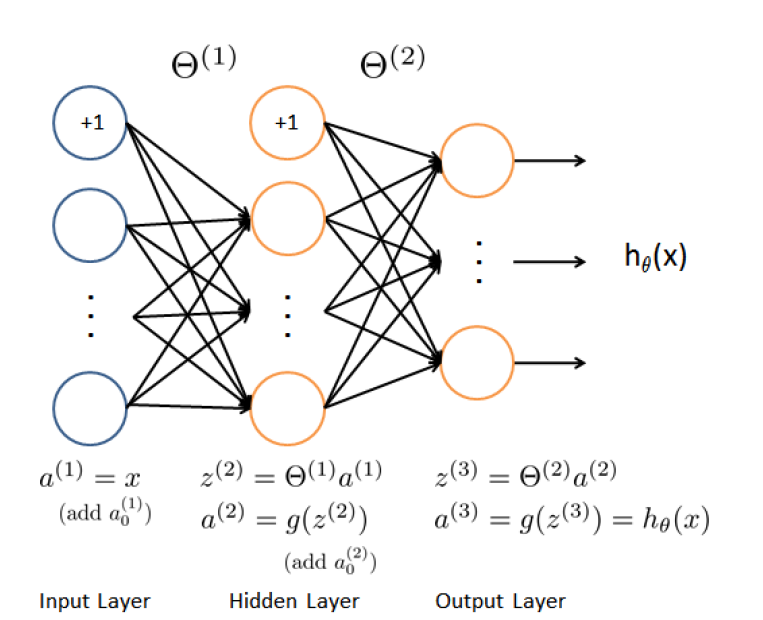
 be the number of inputs(images in our case), and
 ![\[\begin{aligned}J(\theta) = \frac{1}{m} \sum_{i=1}^{m} \sum_{k=1}^K &[-y_k^{(i)}\log(h_{\theta}(x^{(i)})k) \\ &- (1-y_k^{(i)}) \log(1-(h{\theta}(x^{(i)})_k)) ]\end{aligned}\]](https://sisitang0.com/wp-content/ql-cache/quicklatex.com-95b682a68119805c7e43fb53a938c366_l3.png "Rendered by QuickLaTeX.com")
![\[\begin{aligned}J(\theta) = \frac{1}{m} \sum_{i=1}^{m} \sum_{k=1}^K [-y_k^{(i)}\log(h_{\theta}(x^{(i)})k) \\ - (1-y_k^{(i)}) \log(1-(h{\theta}(x^{(i)})k)) ] \\+\frac{\lambda}{2m} [ \sum_{j=1}^{25} \sum_{k=1}^{625} (\Theta_{j,k}^{(1)})^2 + \sum_{j=1}^{2}\sum_{k=1}^{25} (\Theta_{j,k}^{(2)})^2 ]\end{aligned}\]](https://sisitang0.com/wp-content/ql-cache/quicklatex.com-87cd4d2fa66827901a46599c732cec1b_l3.png "Rendered by QuickLaTeX.com")
 uniformly in the range
 ![[-\epsilon,\epsilon]](https://sisitang0.com/wp-content/ql-cache/quicklatex.com-7ff61caddbb05b30248aa8627228858c_l3.png "Rendered by QuickLaTeX.com") . We use
. We use  . This range of values ensures that the parameters are kept small and makes
  is to base it on the number of units in the network. A good choice of
  , where
  and
and  are the number of units in the layers adjacent to
  , we will first run a “forward pass” to compute all the activations throughout the network, including the output value of the hypothesis
  . Then, for each node
  in layer
  , we would like to compute
 that measures how much that node was responsible for any errors in our output.
 (since layer 3 is the output layer). For the hidden units, we can compute
  based on a weighted average of the error terms of the nodes in layer
  .
.
 and place steps 1-4 below inside the for-loop, with the t-
 to the t-th training example
  . Perform a feedforward pass (Figure ??), computing the activations
  for layers 2 and 3. Note that we need to add
  term to ensure that the vectors of activations for layers
  and
and  also include the bias unit.
 in layer 3 (the output layer), set
![\[\delta_k^{(3)} = (a^{(3)}_k - y_k)\]](https://sisitang0.com/wp-content/ql-cache/quicklatex.com-fb4efba4a610f72a23ccf90bb06fe1aa_l3.png "Rendered by QuickLaTeX.com")
![y_k \in [0,1]](https://sisitang0.com/wp-content/ql-cache/quicklatex.com-43d6aac4c83bdd80e54bd70d79563214_l3.png "Rendered by QuickLaTeX.com") indicates whether the current training example belongs to class k (
indicates whether the current training example belongs to class k ( ), or if it belongs to a different class (
 ).
). , set
, set ![\[\delta^{(2)} = (\Theta^{(2)})^T \delta^{(3)} .* g'(z^{(2)}).\]](https://sisitang0.com/wp-content/ql-cache/quicklatex.com-e6ef7efae285319718b9a8889a7bc704_l3.png "Rendered by QuickLaTeX.com")
 .
.![\[\Delta^{(l)} = \Delta^{(l)} + \delta^{(l)}(a^{(l)})^T\]](https://sisitang0.com/wp-content/ql-cache/quicklatex.com-51346ce717c9db9993388fc414e8052b_l3.png "Rendered by QuickLaTeX.com")
![\[\frac{\partial}{\partial \Theta_{ij}^{(l)}} J(\Theta) = D_{ij}^{(l)} = \frac{1}{m} \Delta_{ij}^{(l)}\]](https://sisitang0.com/wp-content/ql-cache/quicklatex.com-6e0480d9edba9d5f80d0f7a48d671f00_l3.png "Rendered by QuickLaTeX.com")
 using backpropagation, we should add regularization using
 ![\[\frac{\partial}{\partial \Theta_{ij}^{(l)}} J(\Theta) = D_{ij}^{(l)} = \frac{1}{m} \Delta_{ij}^{(l)},\quad \mbox{for} j = 0.\]](https://sisitang0.com/wp-content/ql-cache/quicklatex.com-2fb2888b89372f6280caa7ad74f070dc_l3.png "Rendered by QuickLaTeX.com")
![\[\frac{\partial}{\partial \Theta_{ij}^{(l)}} J(\Theta) = D_{ij}^{(l)} = \frac{1}{m} \Delta_{ij}^{(l)} + \frac{\lambda}{m}\Theta_{ij}^{(l)}, \quad \mbox{for} j \geq 1.\]](https://sisitang0.com/wp-content/ql-cache/quicklatex.com-cad92adf13817f57bc07177bc5b365de_l3.png "Rendered by QuickLaTeX.com")