Sisi – Sisi Tang

June 15, 2025June 15, 2025

EFP

EFP is shorthand for Exchange for Physical.

It refers to selling a futures contract and buying an OTC forward or physical metal.

Futures are usually physically settled, while forwards are typically cash settled. The term “Exchange for Physical” might sound misleading here, because by selling futures and buying forwards, you’re effectively exchanging a physically settled instrument for a cash-settled one. Shouldn’t it be called “Exchange for Cash” instead?

Not necessarily. EFP doesn’t refer to the trading venue. It’s a legacy term from the early days of metals trading, when physical metal dominated the market and futures were relatively new. So, when someone moved out of their physical metal inventory and into futures, the transaction was called an Exchange for Physical.

What does EFP short mean?

It means long future and short OTC forward or physical metal. It is the opposite of EFP.

What does negative EFP mean?

In the precious metals market, OTC forwards are traded through the LBMA (London Bullion Market Association), while futures are traded on COMEX (Commodity Exchange Inc., a division of the CME Group).

Under normal conditions, the futures price is higher than the forward price because futures require margin payments and exchange fees. This price difference can be seen as a liquidity premium, since exchange-traded contracts typically offer higher volume and greater liquidity.

A positive EFP means the normal market where future > forward.

A negative EFP means the opposite: future < forward.

In the case of precious metal, negative EFP means LMBA outperforming COMEX.

It is the opposite if you interpret it in a mathematical way. If EFP = forward – future, should EFP negative mean forward < future? No! “EFP negative/positive” is jargon in trading, don’t even think about math.

February 18, 2023February 18, 2023

Toy interest rate curve calibrator

toy-curve-calibrator Download

The attachment contains a toy RFR (e.g. SOFR, ESTR) )curve calibrator and a Libor-type pricer.

It is called a toy because the day count convention and effective/settlement date are not accurately considered. Also, the fine structure of the front end of the RFR curve (short tenors) is not handled. To handle front-end fine structure, short maturity instruments should be used as calibration instruments for example FRA (forward rate agreements). In this toy example, only par swap rates are used.

A key part of an interest rate calibrator is an optimizer or a solver (bootstrapping case only). In this toy example, Excel Solver is used. This is a widely available tool as long as you have Excel. See the Microsoft help page for how to turn on Solver: Load the Solver Add-in in Excel.

Note 1: The calibrator part is set up for a swap whose floating leg pay frequency is annual only, e.g., ESTR and SOFR, because the cashflows are evaluated out of 1-year forward rate. If you were to strip a Libor curve, you have to make the tenors granular enough to cover every payment (every quarter in the Libor case) and add more interpolation pillars.

Note 2: The RFR rate is compounded daily. The actual interest rate paid is a backward-looking backward rate. But it is still reasonable to use a forward rate to evaluate cashflows because any compounding format describes borrowing money for a certain period. The key variable that drives the whole curve is the discount factor, which could be equivalently expressed as forward rate, zero rate, etc.

February 14, 2023February 15, 2023

Black’s Model for Swaption

The quoting convention of the swaption volatility is annualized normal vol under annuity measure. Here, normal is contrary to log-normal. It is also called Black’s (vs Balck-Scholes) or Bachelier’s model. We will use formulas to explain what it means.

Note 1: Black’s model is used for quoting only in modern financial modeling. It doesn’t mean the dynamics of interest rates are modeled this way. A commonly used model for swaption is SABR (stochastic alpha beta rho).

Note 2: The formula below ignores nuances of the effective date, settlement date, and day count convention.

Notations:

$\hat{T}$ : maturity of swaption

$\Delta$ : tenor (maturity) of the underlying swap

$\mathbb{Q}$ : risk neutral measure

$A$ : annuity or annuity measure where annuity matches the floating leg pay frequency of the underlying swap

$K$ : strike

$P(0,t)$ : discount factor from $t (t \ge 0)$ to $0$

$S_{t}(\hat{T}, \hat{T}+\Delta)$ : par swap rate for a swap contract from $\hat{T}$ to $\hat{T}+\Delta$ seen at $t$ . We define a short-hand $S_t := S_t(\hat{T} - \hat{T}+\Delta)$ when there is no confusion.

$\mathbb{E}_t^{\mathbb{P}}$ : conditional expectation on $\mathcal{F}_t$ for filtration $(\Omega,\mathcal{F}, (\mathcal{F}_t)_{t\ge 0},\mathbb{P})$

$PV_{\mbox{something}}$ : present value of something.

$V_{\mbox{something}}(t)$ : value of something at time $t$ .

Below, we set up the formula for PV of a payer swaption assuming the notional is $1. For a more general notional, just scale the formula up by the notional. In a payer swaption, the purchaser has the right but not the obligation to enter into a swap contract where they become the fixed-rate payer and the floating-rate receiver.

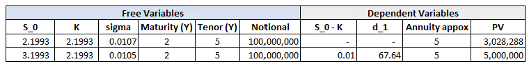
$\small \begin{aligned} PV_{\mbox{payer}} =& \mathbb{E}_0^{\mathbb{Q}}\left[\left(V_{\mbox{float}}(\hat{T})-V_{\mbox{fixed}}(\hat{T})\right)^+P(0,\hat{T})\right] \\ =& \mathbb{E}_0^{\mathbb{Q}}\left[ \left(S_{\hat{T}}(\hat{T},\hat{T}+\Delta)A(\hat{T})-KA(\hat{T})\right)^+P(0,\hat{T})\right] \\ = & A(0) \mathbb{E}^{A}_{0} \left[\left(S_{\hat{T}}(\hat{T},\hat{T}+\Delta) - K\right)^+\right] \end{aligned}$

The last line of the above formula is a change of numeraire from risk-neutral measure to annuity measure.

Since swaption vol is quoted as Bachelier’s vol in annuity measure, the dynamic of interest rate under this measure is the following:

$\small \textrm{d} S_t = \sigma \textrm{d} W_t,$

where $W_t$ is a standard Brownian motion under annuity measure and $\sigma$ is constant.

Hence (by integrating both sides from $0$ to $\hat{T}$ ), denoting by $\mathcal{N}(\mbox{mean}, s.d.)$ a normal distribution, we have

$\small S_{\hat{T}} \sim \mathcal{N}(S_0, \sigma\sqrt{\hat{T}}).$

After plugging in the Gaussian density, the annuity measure expectation becomes

$\small \begin{aligned} & \mathbb{E}^{A}_{0} \left[\left(S_{\hat{T}} - K\right)^+\right] \\ = & \int_{K}^{+\infty} (x-K) \frac{1}{\sigma \sqrt{2\pi\hat{T}}} e^{-\frac{(x-S_0)^2}{2\sigma^2\hat{T}}} \textrm{d} x \\ = & \sigma \sqrt{\hat{T}} \cdot \varphi (d_1) + (S_0 - K) \cdot \Phi(d_1) \end{aligned} ,$

where

$\varphi$ is the probability density function of the standard Gaussian distribution

$\Phi$ is the cumulative density function of the standard Gaussian distribution

$d_1 := \frac{S_0 - K}{\sigma \sqrt{\hat{T}}}.$

Finally,

$\small PV_{\mbox{payer}} = A(0) \left[\sigma \sqrt{\hat{T}} \cdot \varphi (d_1) + (S_0 - K) \cdot \Phi(d_1) \right]$

The Greeks are as follows:

Delta = $A(0) \Phi(d_1)$

Vega = $A(0) \varphi(d_1) \sqrt{\hat{T}}$

Gamma = $A(0)\frac{\varphi(d_1)}{\sigma \sqrt{\hat{T}}}$

The vega-gamma relationship is:

$\small \mbox{Vega} =\hat{T}} \sigma \mbox{Gamma}$

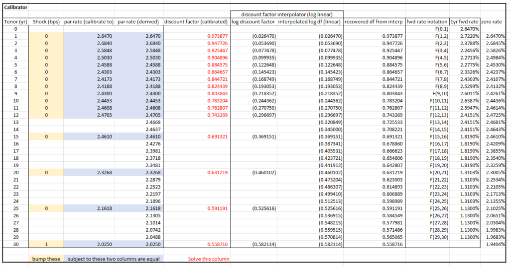
The value of annuity $A(0)$ depends on discounting curve, but one can approximate it by tenor ( $\Delta$ ) in years, i.e., no discounting. The swaption Bachelier’s/normal/Black’s vol is quoted in the unit of bps. For example, 107 means 107bps, i.e., 0.0107. Below we provide two examples of PV: one ATM and one ITM.

For a receiver swaption, PV and greeks can be calculated in the same manner.